The Importance of Out-of-Sample Tests and Lags in Forecasts and Trading Algorithms
I recently had the opportunity to listen to some great minds in the area of high-frequency data and trading. While I won’t go into the details about what has been said, I wanted to illustrate the importance of proper out-of-sample testing and proper variable lags in potential trade algorithms or arbitrage models that has been brought up. This topic can also be generalized to a certain degree to all forecasts. The following example considers a case where some arbitrary trading algorithm is being tested: first without any proper tests, then with proper variable lags, and lastly using out-of-sample methodology. I already downloaded the data (returns for all DJIA-components from 2010 to mid-sept 2016) and uploaded it to my github-page. We can load the data like this:
library(data.table)
url <- "https://raw.githubusercontent.com/DavZim/Out-of-Sample-Testing/master/data/djia_data.csv"
df <- fread(url)
df[, date := as.Date(date)]
0. The “Algorithm”
Say we have a simple algorithm that is supposed to predict the return of some stock (in this case AAPL) with some exogenous inputs (such as returns of other stocks in the Dow-Jones Industrial Average Index) using a linear model (not very realistic, but it serves the purpose for now). We would take a long position if our model predicts positive returns and a short position otherwise. If we control neither for out-of-sample, nor for lags, we receive a portfolio development which would look like this, pretty exciting isn’t it?!
library(ggplot2)
library(scales)
# copy the data
df_none <- copy(df)

# train the model
mdl1 <- lm(AAPL ~ ., data = df_none[, !"date", with = FALSE])

# predict the values (apply the model)
df_none[, AAPL_fcast := predict(mdl1, newdata = df_none)]

# calcaulate the earnings for the algorithm
df_none[, earnings := cumprod(1 + ifelse(sign(AAPL_fcast) > 0, AAPL, -AAPL))]

# plot the data
ggplot(df_none, aes(x = date, y = earnings)) +
  geom_line(color = "#762a83") +
  labs(x = "Date", y = "Earnings Multiple", title = "No Proper Tests") +
  theme_light() +
  scale_y_continuous(labels = comma)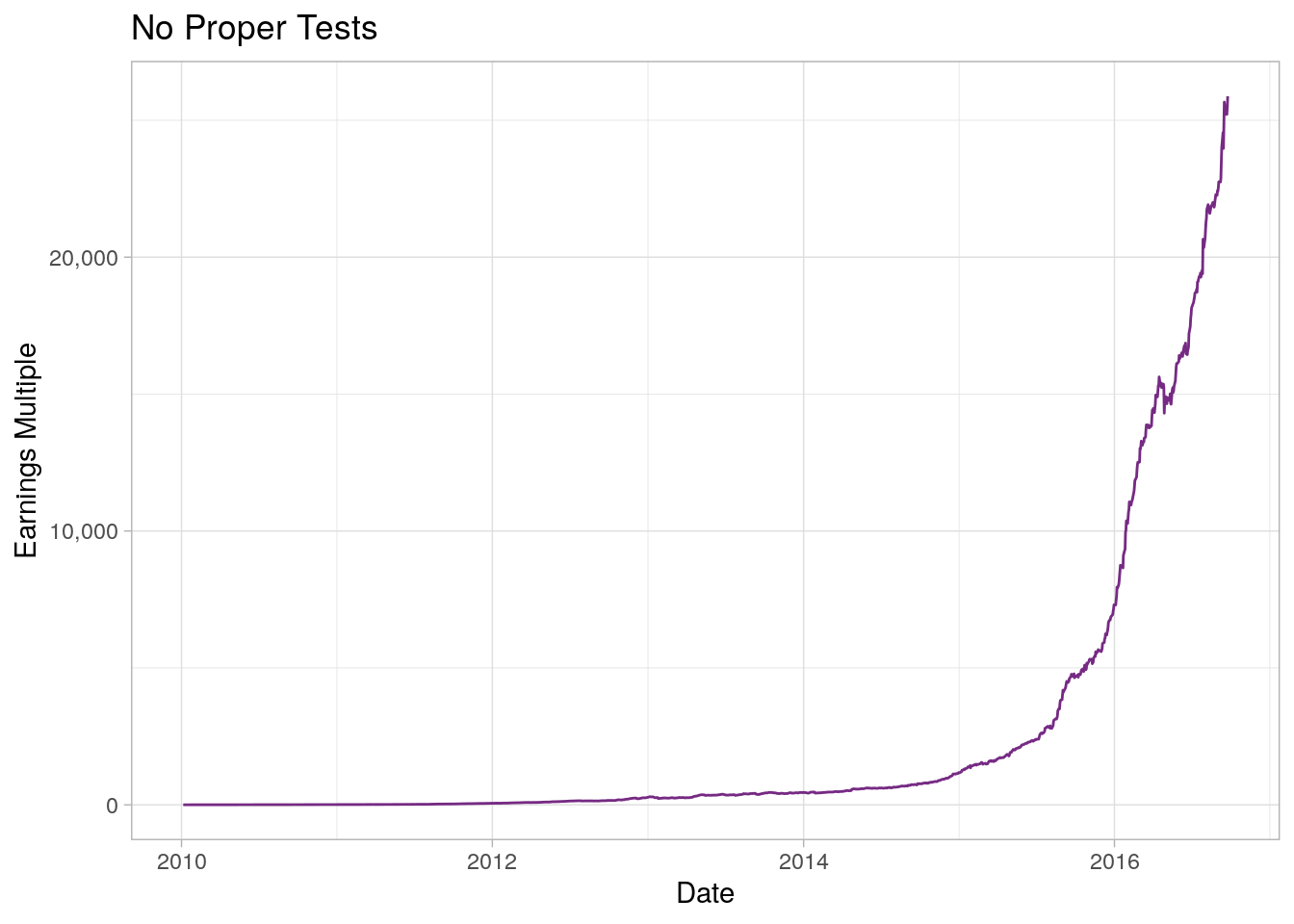
Something’s fishy! I wouldn’t expect a trading algorithm based on a simple linear regression to turn USD 1 initial investment into USD 25,876.65 after 6 years. Why does that performance seem so wrong? That is because an algorithm at the time of prediction wouldn’t have access to the data that we trained it on. To simulate a more realistic situation we can use lags and out-of-sample testing.
1. Lags
The key idea behind using lags is, that your trading algorithm only has access to the information it would have under realistic conditions, that is mostly, to predict the price of the next time unit \(t + 1\), the latest information the algorithm can possibly have is from the current time unit \(t\). For example, if we want to predict the price for tomorrow, we can only acces information from today. To backtest our strategy, we will have to make sure that the algorithm sees only the lagged exogenous variables (the returns of all the other DJIA-components). To save us some time, we can also take the lead of the endogenous variable as this is equivalent to lagging all other variables (except for the date-variable in this case, but that matters only for the visualization).
# copy and clean the data and calculate the lead
df_lag <- copy(df)
df_lag[, AAPL := shift(AAPL, type = "lead")]
df_lag <- na.omit(df_lag)

# train the model
mdl_lag <- lm(AAPL ~ ., data = df_lag[, !"date", with = FALSE])

# predict the new values
df_lag[, AAPL_lead_fcst := predict(mdl_lag, newdata = df_lag)]

# compute the earnings from the algorithm
df_lag[, earnings_lead := cumprod(1 + ifelse(sign(AAPL_lead_fcst) > 0,
                                             AAPL, -AAPL))]

# convert into a data format that ggplot likes
df_plot <- df_lag[, .(date, AAPL_earnings = cumprod(1 + AAPL),
                      earnings_lead)]
df_plot <- melt(df_plot, id.vars = "date")

# plot the data
ggplot(df_plot, aes(x = date, y = value, color = variable)) +
  geom_line() +
  labs(x = "Date", y = "Earnings Multiple", title = "Lagged Variable") +
  scale_color_manual(name = "Investment", labels = c("AAPL", "Algorithm"),
                     values = c("#1b7837", "#762a83")) +
  theme_light()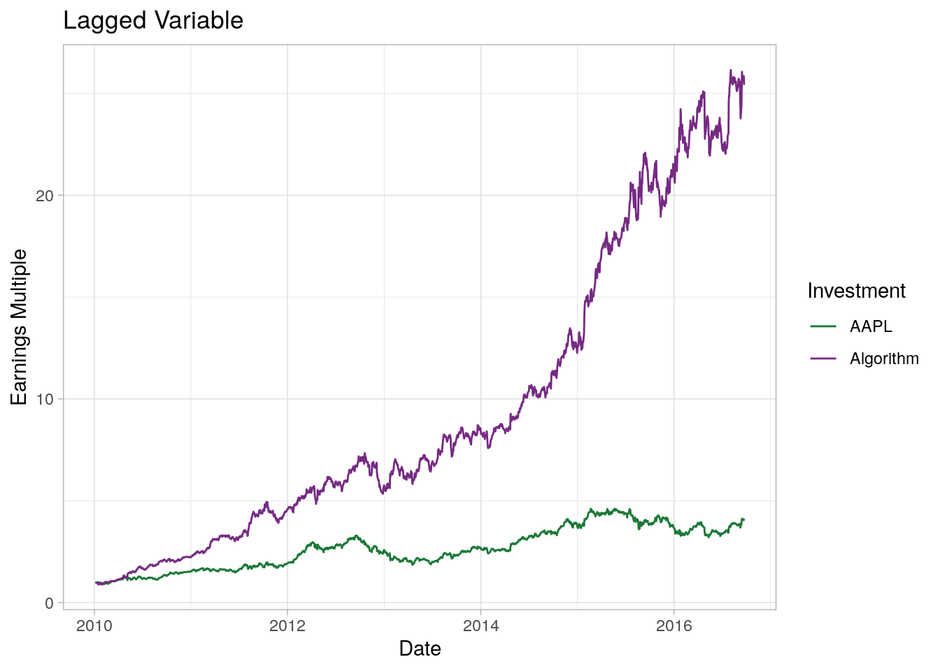
That looks a bit more reasonable, though still unrealistic. The algorithm outperforms the Apple stock by some magnitude of 6; an investment of USD 1 “only” gets turned into 25 (an annual growth rate of rougly 60%). This unreasonable high return is due to the fact that we still haven’t conducted a proper out-of-sample test.
2. Out-of-Sample Testing
So far we have trained the model (or specified if you wish) on the same dataset that we validated the quality of the algorithm on. On a meta-level you can think that the information which we use to test the algorithm is already used in the model, thus the model is to a certain degree a self-fulfilling prophecy (to a certain degree, this is also related to the concept of overfitting). To avoid this, we can split the dataset into two samples for training and validation. We use the training dataset to train the model and the validation dataset to test the algorithm “out-of-sample”.
# copy and clean the data
df_oos <- copy(df)
df_oos[, AAPL := shift(AAPL, type = "lead")]
df_oos <- na.omit(df_oos)

# split the data into training and validation sample
splitDate <- as.Date("2015-12-31")
df_training <- df_oos[date < splitDate]
df_validation <- df_oos[date >= splitDate]

# Train the model on the training dataset
mdl3 <- lm(AAPL ~ ., data = df_training[, !"date", with = FALSE])

# In Sample (for comparison and plotting only) - NOT the out-of-sample test
df_training[, AAPL_fcast := predict(mdl3, newdata = df_training)]
df_training[, earnings_is := cumprod(1 + ifelse(sign(AAPL_fcast) > 0,
                                                AAPL, -AAPL))]

# melt into a data format that ggplot likes
plot_df_is <- df_training[, .(date, AAPL = cumprod(1 + AAPL),
                              algorithm = earnings_is)]
plot_df_is <- melt(plot_df_is, id.vars = "date")
plot_df_is[, type := "insample"]

# Out-of Sample Test
df_validation[, AAPL_oos_fcast := predict(mdl3, newdata = df_validation)]
df_validation[, ':=' (
  earnings_oos_lead = cumprod(1 + ifelse(sign(AAPL_oos_fcast) > 0,
                                         AAPL, -AAPL))
)]

# melt into a data format that ggplot likes
plot_df_oos <- df_validation[, .(date,
                                 AAPL = cumprod(1 + AAPL),
                                 algorithm = earnings_oos_lead)]
plot_df_oos <- melt(plot_df_oos, id.vars = "date")
plot_df_oos[, type := "oos"]

plot_df <- rbindlist(list(plot_df_is, plot_df_oos))

# plot the data
facet_names <- c("insample" = "In-Sample", "oos" = "Out-of-Sample '16")

ggplot(plot_df, aes(x = date, y = value, color = variable)) +
  geom_line() +
  labs(x = "Date", y = "Earnings Multiple",
       title = "Lagged Variable + Out-of-Sample Test") +
  scale_color_manual(name = "Investment", labels = c("AAPL", "Algorithm"),
                     values = c("#1b7837", "#762a83")) +
  theme_light() +
  facet_wrap(~type, scales = "free", labeller = as_labeller(facet_names))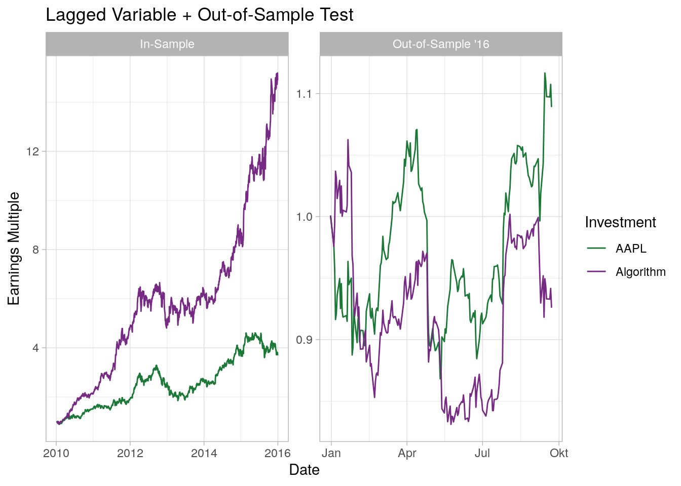
As expected, the algorithm returns less than the stock it matches against (AAPL). If we would invest in this simple algorithm, I would expect our investment to go down a lot more. All of this is of course without considering trading, execution, and other transaction costs, which would even further decrease the returns of our trading algorithm. To sum it up: If you are looking into algorithms and/or forecasts, always make sure that you apply proper out-of-sample tests and think about what information could have been used at the time of decision to avoid overfitting. As always, if you find this interesting, find an error, or if you have a question you are more than welcome to leave a reply or contact me directly.
David Zimmermann, PhD
Data Scientist
I am an economist by training, turned programmer/data scientist who loves to program with R, Python, and C++.